In the previous article we tried to analyze what is the Contrast Ratio in a LED driver and how the non-idealities are giving a boundary on the minimum allowable PWM period. That was quite worth a full article, but a big part was indeed missing.

Here we will go through how the PWM period and the non-idealities are related to each other. From this, how a final PWM requirement can be derived directly from the non-ideal average current.

In many application notes the slew rate of the output of some drivers is overlooked, due to the fact that is assumed to have a driver working properly, by trustfully following what has been implemented by the application engineer. Often, is just treated the most important aspect of the output ripple, but is not always the only aspect. Let’s take into consideration the case of a constant driver Infineon ILD4001 and its related AN213. The question is, if a product shall be optimized and analyzed, how much closely one should follow the reference design? The AN does not talk about rise and fall times of the output driver, rather “only” about the current ripple. Sometimes, may be worth to just check if an optimization is possible by looking at other less dramatic non idealities, to push a device to its boundaries, while cross checking the tradeoffs.

The average current is a lie

As stated in the previous article, the PWM frequency must be higher than the minimum on-time of the converter, including the time to turn on and off when the control signal tells the driver to turn off, in order to reach both the full-on and the full-off state:

     (1)

But at this limit, there is practically no duty cycle exploitable, since any less duration will not bring enough time to fully reach the programmed output. In fact, from the moment in which the PWM duty cycle, at this fast frequency, goes from 100% to somewhere below, the actual peak average dimming level cannot be precisely controlled since the driver does not have the time to fully turn on or fully turn off, or even both. Why this? Because usually it is used a DC-DC constant current driver, which uses an inductor to provide the current and by definition such inductor with a constant voltage applied, will have a current which increase and decrease with certain linear slopes, assumin no saturation occurs.

The Figure 1 is worth a thousand words, showing a Duty Cycle scenario when dealing with dimming PWM frequency which is too high with respect to the rise and fall times of the current slopes in red, in 3 possible dimming situations, to explain the previous paragraph. It is also shown again what are the and . Please note that this is not the DC-DC PWM, but the slower dimming PWM commonly used in LED systems.

It is therefore important to know the slew rate when the PWM period is too short. Too short that the on and off time will be comparable with the duration of the slope relative to the current. But will this be a problem? Can I push the limits of the dimming PWM frequency?

Let’s try to model this current to derive the control requirements. But before, here is mentioned the driver used to model the current.

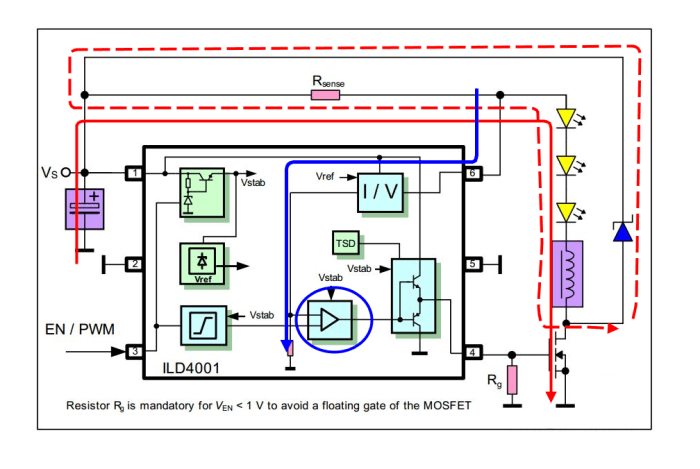
A relatively simple circuit topology: hysteretic buck converter

This architecture (an ILD4001 driver), with a fully on signal, turns on the MOSFET, thus charging the inductor, up to when a certain control voltage is reached, then turn all off thus discharging the inductor down to when a lower threshold in the control voltage is reached. Therefore does not have a fixed timing and the frequency and duty cycle (this time the DC-DC one, not the dimming one) varies with load and supply. On the other side, this architecture helps in dealing with PWM requirements very easily and being a simple one, may be more dependable and bring cheap designs. Here a basic schematic of such circuit is shown:

From the topology to the true average current calculation

In the following equations, from the Figure 2, is the supply voltage. Also, let’s assume as the forward voltage of our LED strip and the free-wheeling diode drop.

Here I will neglect the inductor parasitic resistance, which somehow bring the same effect of concerning the RL time constant. This is a side-effect hidden in the slopes, which are on their own a side effect of the normal use case of the driver. The RL time constant alters the linearity of the ramp, where for this theoretical approach can be totally neglected. – If it can’t be neglected, then there is a more serious problem with sense resistor and inductor sizing.

When the inductor charges (MOSFET on), will provide a current with a certain positive slope:

     (2)

When discharge (MOSFET off), there will be a negative slope:

     (3)

Another important thing to take into consideration is that a generic current ramp increase of a quantity which is the slope of such current times the amount of time in which this slope is applied.

The current peak, as can be understood by looking a Figure 1, is the result of the slope multiplied by the time in which this slope exist (assuming to be short enough to have no core saturation of the inductor). Therefore current highest value limited by the driver is , because of course, is a constant current driver. Now, when describing such drivers, is often used as a characterization parameter the time to go from to as and viceversa to as :

   (4)

Where is the time required to reach from no current (see Figure 1). If the current reached is lower, let’s call it , the consequence the slope duration is lower and does not represent the full current swing anymore, therefore is not anymore the . So let’s call this instead since is happening during the on-time:

   (5)

which may be or not equal to .

For simmetry, if the lost during the off-time is equal to , then the off-time will be :

   (6)

Again, if this current is lower, the duration of the slope does not represent the full current swing anymore, so can be renamed as :

   (7)

From this basic concept can be found few different scenarios in which the current behaves and affect the average current, depending on the PWM period and duty-cycle.

Modelling the average current

We are dealing with triangle waveforms with rise and falling slopes; and also with rectangle and trapezoidal shapes, as can be seen later here. Therefore few cases must be considered. Also, a more general one will be derived out of basic simple models.

Example 1:

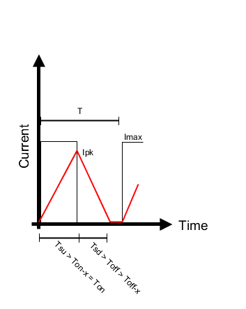
This is a very bad scenario. The driver used in these conditions is all but predictable and the proper dimming performance is completely out of linearity. Here I will show this on numbers.

The current rises with a slope, with a duty cycle so short that makes it impossible to reach the maximum value, stopping at . In this case, only for simplicity consider the off-time to be long enough to let the current reach 0 after . It will be considered later.

Let’s call instead of because the time in which the current actually rise never reach the maximum, so the duration is lower. Then is needed to exclude the driver’s delay   which delays the start of the ramp (not shown in the picture). While the is, in this case, just the duration of the falling ramp and again is not because is shorter, since the starting point is not the but a lower peak .

        (8)
         (9)

The duration of the falling slope is , from the , is:

         (10)
       (11)

From the average value of a triangular signal, with time on x-axis and current on y-axis, the average current is:

      (12)

Where is the PWM period. Filling in the previous terms:

     (12a)

Now if for simplicity we set the ramps as equals, and neglect the delay of the driver to have , where with being the PWM frequency. From (12a), collecting and simplifying , the current became:

Which means:

   (13)

The simplified result in eq. (13) is also intuitive: with the rise slope constant, since is imposed by the hardware, the average current is proportional to the square of duty cycle. Also, is the , so is also proportional to this. Because extending the duty cycle we are extending the base of the modelled triangle due to higher peaked current, the area should increase by a factor proportional to the square of such base length increase, but still averaged out on the period. So this situation is all but linear and controllable.

This model works only if the current waveforms are triangle, therefore is valid up to the moment the ramp will increase to the maximum current allowed by the driver, and not anymore. Also, the time of the PWM shall be long enough to let the current go to 0 (zero), so keeping the triangular shapes, as per thi Example 1 in Figure 3. Therefore the Example 1 is valid if the following conditions are true:

   (14)

When the PWM changes so that the conditions (14) become false, is needed to model another example.

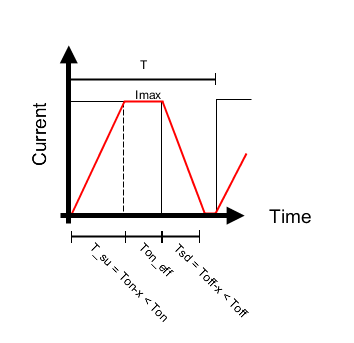
Example 2:

This case is still a representation of a bad PWM frequency selection, but the result is an higher average current than expected and very limited duty-cycle dynamics. This happens from the moment in which the condition (14) is not true anymore.

Here the area calculation principle is the same, but it is not anymore only made by two triangles rectangles. Because there is also the area in which the current is , of duration . The result is an additional term to average out the constant current of duration . By adapting the same equations used before and considering the Figure 4:

     (15)
         (16)

Now the falling ramp starts from the maximum current and not the lower peak current , as in Figure 3. Then, the duration of the falling time became, according to the Figure 4 is:

     (17)

Because and the duty cycle is decided by the designer, we have now all the variables to find the average current:

     (18)

Trying to simplify a bit the term of the triangle area by neglecting , is possible to obtain:

     (18a)

Regarding the ramps, now the maximum current and their slopes are design dependent, and if their contribution is large, a slow rising/falling slope with a high maximum current, due to its square term, can produce a high contribution. The Example 2, as can be conceived from the picture, holds only if the rise slope lead to an higher current than the maximum, thus needing the regulator to activate to limit within . Also, to represent this scenario, need to be longer than the duration of the falling slope. As a result, the Example 2 holds as long as the follwing conditions are true:

   (19)

But now, if and are deeply different, and the falling slope is slow enough to not let the driver completely turn off the output, there is a memory, thus the conditions for eventual transients which are adjusting after few PWM cycles. This requires a new big scenario. But this may also not be a complete description of all possible combinations of ramps and duty-cycles: there is the need to describe a more general case.

A complete scenario

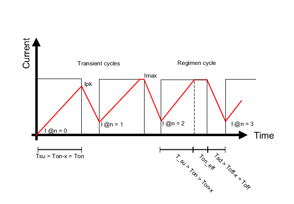
In this Figure 5, after the first cycle, the PWM period is so short to not let the current completely extinguish during the off-time, the next cycle will start from an higher current (I@n = 1). This lead to a transient event (transient cycles in Figure 5), which then will eventually stabilize over time (regimen cycle).

To properly model this situation, let’s take the rise from I@n=0 (herein called ) to . The area is calculated, as just did for Examples 1 and 2, from the area rule of triangle. Here there may be rinsing current from a base higher than 0, so that the law is a rectangle trapezoid, which naturally extends to the triangle shape when one side goes to 0. Defining peak current as the final current after the on-time and including a delay time from input to output of the driver:

       (20)

Considering that the driver will correctly limit any current up to , the increase of the current to reach the peak will be bound within the maximum current in magnitude, and within the on-time in duration, so we can redefine:

       (21)

As a result, when the ramp takes requires more time than to arrive at , then  the limit will be (take a look at the first period in Figure 5). The conclusion is that the peak current can be found under certian boundaries imposed by the physics or the DC-DC driver. Here the generalization over samples apply, so instead of , is used the generic , with the help of a binary coefficient to keep limited:

       (22)

Now the average rising current is the area of the trapezoid shape of the current path on the time axys (see Figure 5), divided by the duration of the PWM period:

   (23)

If , there is also a constant current contribution. By defining the term as:

   (24)

The constant current contibution, with the help of the same binary coefficient , became:

     (25)

The falling, like the rising, will follow a trapezoidal shape, will start from to the next current sample I @n=1 from Figure 5, therefore generalized again over samples became:

   (26)

This means that the terms shall be calculated upfront before calculating the average, to take in condieration the term during the step of . The sample generator is just a summation of the initial current, plus the history of rising and falling ramps, which defines the next current sample. But due to the circuit and the physical limits, this shall be again limited within and . Here the generator equation over PWM periods is built in the following way:

(27)

With all the samples, is possible to merge together all the equations and observe if the result tell us something:

    (28)

Extending the terms and the condition of existence:

     (29)

Now, just for the sake of analysis and developing all the terms and , neglecting since it is already quite long and wont change the concept, we have:

The result tell us that by computing the eq. (27) over all the periods, knowing the maximum current of the driver and the PWM signal applied, the eq. (29) can be issued for each cycle, taking into account the hisotry of the previous samples. In this expanded equation is possible to spot a familiar situation with the Example 1, by developing under the conditions to have , therefore eliminating the constant current term and developing the remainig ones. By applying the simplifications made on the two remaining terms we obtain:

which is the same square proportionality with the duty cycle seen in the Example 1. Which means that again, is all but linear. Also, normally you don’t want to have to compute all these equations to know the average current, and by making the ramp time negligible w.r.t PWM periods, all will reduced to

    (30)

keeping all the relations linear.

The slew-rate of the output which drives the PWM requirements

After all this computation, the conclusion is that the best way to use a constan current driver and in general any PWM based system, is to minimize the slew rate of the PWM signal with respect to its period. And here is shown why, in terms of controllability, design times and accuracy. But now, what will be such requirements for a designer or for the controller?

The rise and fall times will just need to be negligible, thus always let the current reach and at each cycle. Therefore, the first step is to define which on and off time can be used while in dimming (otherwise the driver will be always on or always off). Also, the worst cases of rising and falling slew rates will be when they have to achieve the full swing of current:

Knowing that there is a slew-rate when turning on, the minimum on-time will therefore be:

   (31)

while, assuming thedelay time happens only on the on time due to the driver artificial delay (for filtering reasons), the maximum on time is defined by knowing that there is a slew rate when the off time starts:

   (32)

Secondly, is possible to find the minimum PWM period:

     (33)

Because this number is suspiciously low, must be remembered that at the edge ofthis requirement there is no resolution available, because ifthe controller can be precise, the driver will not and instead of the nice (and normally known) eq. (30), we will have to deal with the eq. (29). So the suggestion is to have:

     (34)

This is the basic requirement that is a must. Also, can be virtually very large, except for the flickering effect. At this point, with a working prototype, depending where it is used, a new few problems may enter: the resolution, the precision and how PWM period shall me modified according to the application. This is worth to be discussed in a different article.